Durango Bill's
The Infamous
Traveling Salesman Problem
Traveling Salesman Problem
Wikipedia: The traveling salesman problem asks the following question: "Given a list of cities and the distances between each pair of cities, what is the shortest possible route that visits each city exactly once and returns to the original city?"
“The traveling salesman problem isn’t a problem, it’s an addiction.”
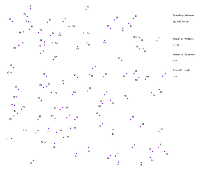
(Click on image for a large version)
The diagram above shows 100 vertices scattered randomly across an X/Y coordinate plane. The distance between any 2 vertices can be easily calculated via:
Distance = sqrt [(difference in X
coords)2 + (difference in Y coords)2]
Assume that the problem is symmetrical – i. e. The distance from any point “A” to point “B” is the same as the distance from point “B” to point “A”.
Suppose you want to find the shortest Traveling Salesman route via the following algorithm:
1) Systematically, generate all possible routes.
2) Sequentially go through your list to find the shortest path.
How long would it take?
Initially, you could start at any defined point (vertex), go to any of 99 other points, then go to any of the remaining 98 points (vertices), etc. until you return to the starting point. The number of possible paths = 99 x 98 x 97 . . . 2 x 1 = 99! = 9.33 x 10155. (Divide by 2 if you don’t care about the travel direction.) (Multiply by 100 if you can start at any point as opposed to a defined point.)
Let’s assume that you would like to have computers help you to do the calculations. There are approximately 1.0E80 atoms in the visible universe. Assume that each of these 100 million billion billion billion billion billion billion billion billion atoms is a computer that can generate a billion possible routes per second. How long would it take these 1.0E80 computers to generate the complete list? The answer is ~3 hundred thousand billion billion billion billion billion billion years.
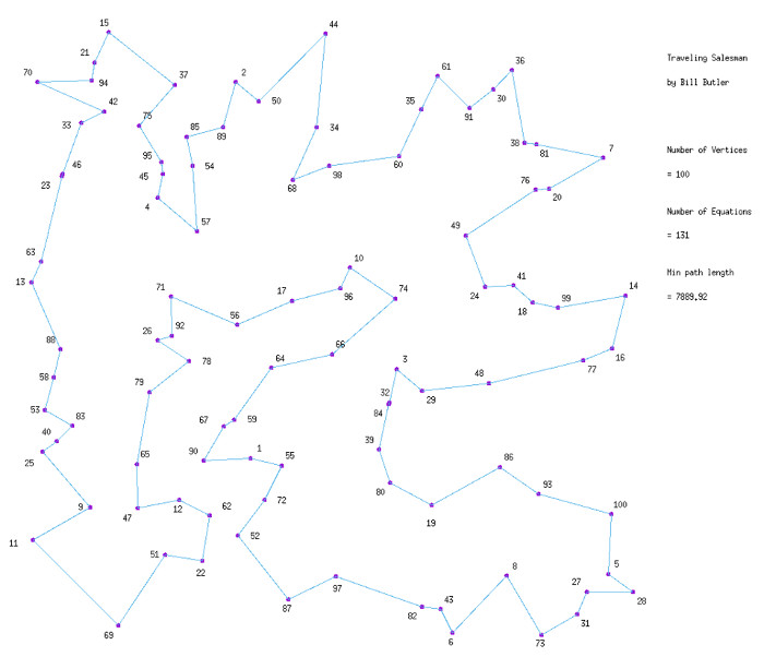
A “somewhat” faster way to find the shortest route is to look at the diagram below.
(Click on image for a large version)
The diagram above shows the shortest possible path to visit each vertex exactly once and return to the starting point. The illustrated path is guaranteed to be optimal.
Finding the shortest path
For the following, the author used his own Linear Programming software (in “C”) with the author’s own Traveling Salesman add-on. No “branch and bound” operations were involved. The diagrams for the results were generated by the (free) “gnuplot” package. All of this was within a Linux operating system. Computer solution time for the final iteration was about 0.01 sec. User time was measured in hours since constraint equation entry was manually tedious.
The “random” vertices were generated with a “pseudo random” number generator on an X/Y coordinate plane. (Pseudo random means the distribution should pass all random number tests, but the results could be identically reproduced for some other program if you initialized the generator with the same seed number.) The scale for the sample problem was 0.0 <= X,Y coordinates <= 1000.0. Coordinates for the vertices were “double” floating point numbers.
In most mathematical problems, the solution process starts with defining what we are looking for. For this problem, we wish to connect the dots (use edges to connect the vertices) in such a way that each dot (vertex) has one “came from” edge and one “goes to” edge. The net result must be one single cycle. There are as earlier mentioned, billions and billions of possible paths. The answer will be the shortest of these billions and billions of paths.
There will be COMBIN(100,2) = 4950 potential edges in this sample problem. Exactly 100 of these will be required for the solution. For mathematical purposes, we will want to derive a value of “1.0” for the edges in the solution and “0.0” for edges that are not in the shortest (minimal length) solution. The final path length will thus be a simple addition of the distances for the “1.0” edges. The path that has the minimal total will therefore be our minimal solution.
Our mathematical solution process will use a combination of Linear Programming (and specifically the “Upper Bound” variation) and topology. Please see the author’s web page titled “Guaranteed Profits in Stock Market Options?” at http://www.durangobill.com/LP_Options.html for another application of Linear Programming.
First, we will need a numerical method of identifying each of the 4950 edges in the problem. The vertices are numbered – and each edge connects a higher numbered vertex to a lower numbered vertex. A unique number for each edge can be easily calculated via:
Edge number = [(Higher – 1) * (Higher – 2)]
/2 + Lower
The following is a small table showing the results for 7 vertices:
Higher
1 2 3 4 5 6 7
----------------------------
L 1 | 1 2 4 7 11 16
o 2 | 3 5 8 12 17
w 3 | 6 9 13 18
w 4 | 10 14 19
e 5 | 15 20
r 6 | 21
The general format of a linear programming problem consists of:
1) Minimize (or maximize) a mathematical expression.
2) Subject to a series of mathematical equations that constrain the results to what is needed to solve the problem.
Part 1 is easy:
Minimize Z = c1x1 + c2x2 + c3x3 . . . c4949x4949 + c4950x4950
The “c’s” in the above equation are the distances (costs/edge lengths) between the vertices, and the “x’s” are the edge identifiers (variables). The “x’s must have a value of 1.0 if the edge is in the solution, and 0.0 if the edge is not in the solution.
Part 2 makes life “interesting” (The previously used word “addiction” could also be used). Formulate a series of mathematical equations such that they:
Constrain the solution so that there will be a series of connected edges (Solution value = 1.0) such that they form a continuous path that solves and minimizes the Traveling Salesman’s path. Edges that are not in the path will have a value of 0.0.
The Upper Bound version of the Linear Programming algorithm makes it easy for all edges to have a maximum value of 1.0. (Linear Programming will automatically assign “0.0” for a lower limit. Trying to eliminate the in-between decimal values for the edges (variables) tends to produce programmer “stress” problems. As in the previously mentioned “addiction” factor.)
The Iterative Solution Steps
The first 100 constraint equations for Step 2 can be easily generated by a computer program. For each of the 100 vertices, the sum of the values for the connecting edges for any vertex must equal 2. There are 99 potential edges (the “x’s”) that emanate from each vertex. 2 of these will have a solution value of 1.0, and the remaining 97 edges will have a value of 0.0. (At least this is what it will look like when the final solution is found.)
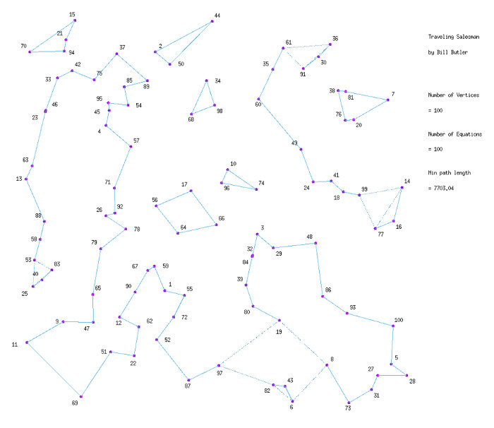
(Click on image for a large version)
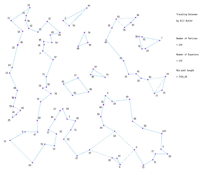
The diagram above shows the computational result for these initial 100 constraint equations. Each edge has an upper bound of 1.0 and the sum of the edges for each vertex = 2.0. The bad news is that there are multiple unconnected cycles. Worse yet, some of the vertices have more than 2 edges. When more than 2 edges exist, at least some of these edges will have decimal values.
But these problems “are not going to trouble us”. What we learn in school is: “Build a better mousetrap and the world will beat a path to your door.” (And what we learn after school is: “Build a better mousetrap and nature evolves a smarter mouse”.)
Iterative Step 1
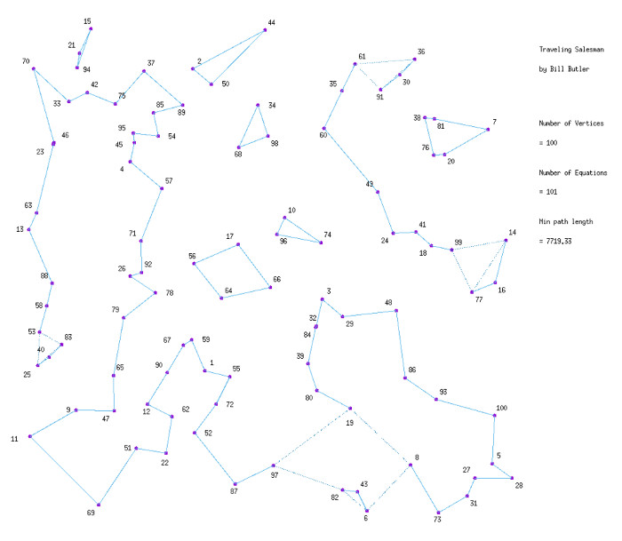
If we look at the complete Traveling Salesman solution shown earlier, we note that if you draw a line around any subset of the 100 vertices, there will be at least 2 edges that cross this encircling line. If we look at the upper left corner of the above diagram, we note that you can draw a line around vertices 70, 15, 21, and 94; but the line will not cross any edges.
We can thus add another constraint equation to our system that says: “The number of edges that cross this enclosing line must be >= 2. A better way of expressing this for a constraint equation is to say: The sum of the edge values that are completely inside this encircling line must be <= 3. (In the interim solution shown above, there are 4 edges that are plotted.) Therefore we add another constraint equation to our system that says:
The sum of the values of the edges that are internal to vertices 70, 15, 21, and 94 must be <= 3. The general form for these cycle equations is that the sum of the interior edge values must be <= (the number of enclosed vertices - 1)
(Click on image for a large version)
After we solve the above system (that now has 101 constraint equations), we get the above diagram. The bad news is that nature has evolved a new way of avoiding the solution that we would like to get. The good news is that, somewhere, there is a legitimate Traveling Salesman solution that has a finite length. We don’t know what this finite length is, but if you check the “Min path length” in these 2 interim solutions, you will see that we are now some 16.29 units closer to an eventual solution.
Iterative Step 2
The upper left corner still has a problem. The constraint equation that we entered for vertices 70, 15, 21, and 94 did produce a pattern that intersects two edges (the edges that now connect vertex 70 to other vertices), but vertices 15, 21, and 94 form a separate cycle. The next step is to generate another constraint equation that says the sum of the values of the internal edges for these vertices must be <= 2.
(Click on image for a large version)
The diagram above shows the result of adding a constraint equation for vertices 15, 21, and 94. We still don’t have a Traveling Salesman solution, but we have gained another 4.72 units toward a solution.
As an omen for what is to come, the edge pattern for vertices 70, 15, 21, and 94 has settled into what looks like a stable path for the final complete solution. (Hint: Nature is about to evolve a smarter mouse.) If you compare the above edge pattern for these 4 vertices with the finally solution, the path changes. In the minimal solution, both of the edges from vertex 70 go to other vertices.
After Iterative Step
11
(Click on image for a large version)
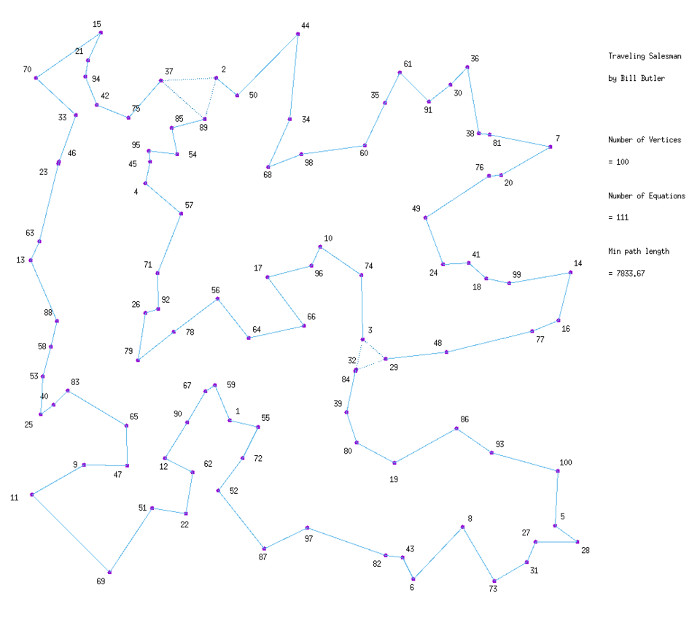
9 more cycle equations produced the above diagram. These 9 additional constraint equations have brought us closer to a legitimate Traveling Salesman solution, but the middle of the diagram reveals a problem. In any T. S. solution, any line that you draw through the diagram will intersect an even number of edges. In the above diagram, its easy to draw a line that intersects 3 edges. (or possibly 5 edges, . . . ) (And it can get a lot worse. Larger problems usually degenerate to where a lot of fractional edge values exist.)
There are also 2 triangles in the diagram with fractional values for their edges. We will look into this problem a little later.
There are no opportunities for the cycle equations that we have been using for new constraint equations, so we must develop a new tool.
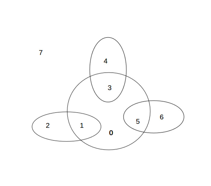
Consider the above 8 Zone diagram. Try to draw a continuous line through the 7 Zones (1 to 7) (Zone 7 is an “everything else outside” zone) and optionally through Zone “0”, and finally return to your starting point. If you count the number of times that you have to cross one of the illustrated lines, you will find that it takes at least 10 line crossings.
Next, imagine that you have one or more vertices in Zones 1 to 7 and optionally others in Zone 0. Try to connect all of these vertices using your continuous line. Experimental results will once again show that you have to cross the given lines at least 10 times.
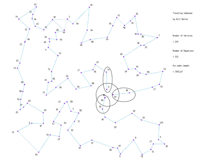
Now, let's superimpose the above diagram on one of the triangle formations that we got after Iterative Step 11. Put vertices 32 and 84 in Zone 1, vertex 39 in Zone 2, vertex 3 in Zone 3, vertex 74 in Zone 4, vertex 29 in Zone 5, and vertex 48 in Zone 6. Everything else falls into Zone 7.
(Click on image for a large version)
Note: Edge values for the dotted lines in the triangles have a value of 0.5.
If you add the values for the edge crossings, the central circle of our 8 Zone diagram will intersect edges with edge values totaling to 3 while each of the 3 ellipses intersects edges with a total value of 2. The total of the intersection values is 9. (In our sample problem, most of the edges are integer “1’s”, but they can just as easily be multiple edges with fractional values. The only thing that counts is that the sum of the edge values is < 10.0) But as our experiments have shown, a complete closed path requires a value of 10.0 or more. We now have a new tool that can be used for additional constraint equations.
The resulting constraint equation is the sum of treating Zones 1 and 2 as a cycle equation; plus Zones 3 and 4 as another cycle equation; plus Zones 5 and 6 as another cycle equation; plus Zones 0, 1, 3, and 5 as another cycle equation.
Note that a larger 8 Zone equation could be used for the triangle pattern at the top of the partial T. S. solution. If we rotate the 8 Zone pattern some 180 degrees, we could put vertex 49 in Zone 1, vertices 24 and 41 in Zone 2, vertex 57 in Zone 3, vertex 71 in Zone 4, vertices 46 and 23 in Zone 5, vertices 63 and 13 in Zone 6, everything above these vertices in Zone 0, and everything else in Zone 7.
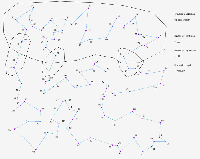
The diagram above shows the 8
zone boundaries if we wanted to use the upper triangle. A
single section of the computer code processes both examples to
generate a constraint equation.
(Click on image for a large version)
If we generate another constraint equation using the first of the above options and then solve the system, we get the above diagram. It’s still not a complete TS solution, but we just drove the total path length up from 7833.67 to 7837.55.
Another 19 constraint equations (using both Cycle and 8 Zone equations) finally produced the sought after minimal Traveling Salesman route. It turns out that 6 of these constraint equations were not needed (Hindsight helps in deciding what really is needed vs. what looked like it might be needed.) Of major significance, no "branch and bound" operations were involved.
As Traveling Salesman problems become larger, the interim solutions degenerate into fractional solutions that can not be solved by just cycle and the simple version of the 8 Zone equations. The good news is that there are multiple more mathematical tools available. There is a whole family of equations similar to the 8 Zone equation. None of these were required for this particular problem.
(Click on image for a large version)
If you look at the solution for this particular (or any) T. S. problem, the solution path splits the graph area into distinct inside and outside parts. Each vertex in a solution has an “inside area” on one side of its edges and an “outside area” on the other side. Constraint equations can be constructed using this property.
At a more advanced level, if we look at the 3 edges that form triangles (could also consider larger polygons), at least one edge of the triangle can not be present in a T. S. solution. At least one of these triangular edges can be (at least temporarily) driven out by taking advantage of the “opportunity cost” equation that is always present in the “Revised Simplex” algorithm. (Each edge in a triangle pattern will have an opportunity cost of 0.0) Thus, generate a constraint equation that sets the sum of these opportunity costs to > 0.0 for these 3 edges. (Would have to calculate the required components of the Simplex Tableau that are subsequently used to derive the 3 relevant coefficients in the current version of the objective (opportunity cost) equation.) Of note: this methodology is a topological constraint equation and not a branch and bound operation.
Closing notes
It is not known if larger Traveling Salesman problems can be solved in polynomial time or if exponential time is required. When topology is used to construct constraint equations (i.e. the 8-Zone and related equations), it appears that the Traveling Salesman problem may be solvable in polynomial time. The author's algorithm/methodology is basically a combination of linear programming and the famous 7 bridges of Konigsberg problem.
The author thinks that T. S. problems will eventually be solved in polynomial time if algorithms that use iterative steps are used instead of just using a fixed set of constraint equations that are formulated before running a computer program, but it is beyond what I can do as an individual. There is a contest between what programmers/operations-research personnel can do in building better mouse traps vs. what mother nature can do in evolving smarter mice. The contest hasn’t been decided yet.
Additional Notes
One possible approach to simplify finding a solution to a T. S. problem might be to just use the edges from a Voronoi Triangularization. (Please see the author’s web page at http://www.durangobill.com/Voronoi/VoronoiDiagrams.html for more information.)
(Click on image for a large version)
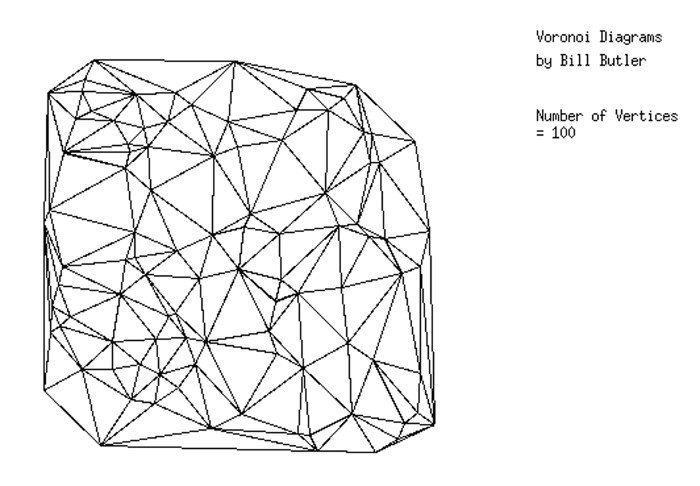
The diagram above shows a Voronoi Triangularization for the same “pseudo random” set of vertices used for this Traveling Salesman Problem. The minimal T. S. solution has an edge connecting vertices 70 and 42 (in the upper left corner).
The Voronoi Triangularization diagram does not include this edge. Most Traveling Salesman solutions will include edges that are not present in Voronoi Triangularizations. (Assume both use the same set of vertices.) Scratch the Voronoi Triangularization hypothesis.
Traveling Salesman
Approximations
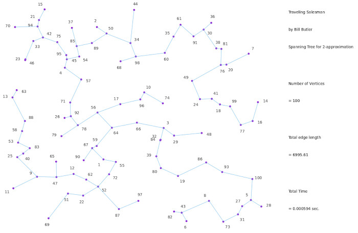
In practice, even if the exact optimal path can be found, it is often difficult and/or time consuming to do so. Thus "close enough is OK" approximations that can be quickly/easily done are frequently used instead. We will take a brief look at 2 of these - the minimum spanning tree/2-approximation algorithm and the convex hull/shrink wrap algorithm.
The Minimum Spanning Tree /
2-approximation Algorithm
A minimum spanning tree is a graph diagram that uses "N - 1" edges/lines to connect "N" vertices/points.
(Click on image for a large version)
The diagram above shows a minimum spanning tree for our 100-vertex sample problem. 99 edges connect the 100 vertices, and do so with the minimum possible total length. Traditionally, the topmost vertex is called the "root vertex".
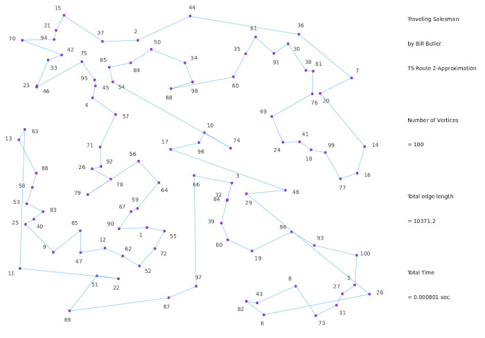
If we start at the root vertex, do a counterclockwise "tree traversal", make a list of visited vertices in the order of the first time they are visited, and finally return to the starting "root vertex" , we will get a closed path that visits all the vertices. As an add-on we have sorted the son/daughter branches to access them in a counter-clockwise sequence. The result looks like the following:
(Click on image for a large version)
The path above does satisfy the requirement of a closed loop that visits all the vertices and returns to the starting point, but it forces a path that is basically a skinny outline of the original spanning tree. The total path length is some 31.45 % longer than the optimal route that we found earlier. This might be sort-of-OK, but maybe if we try a different algorithm, we might get a better result.
The Convex Hull /
Shrink-Wrap Algorithm
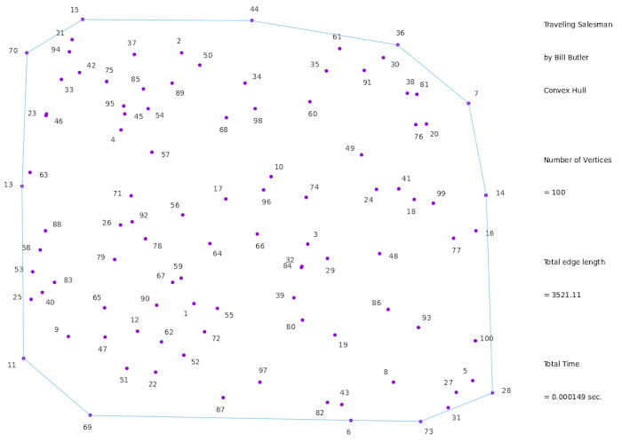
As you might assume by the name, the Convex Hull / Shrink Wrap Algorithm starts with a Convex Hull diagram. If you think of the vertices as pegs in a peg board, and then wrap a string around the pegs, the result would look something like the following:
(Click on image for a large version)
The diagram above shows the convex hull for our 100 vertices. It can be generated by the following computer pseudo-code.
1) Find the vertex with the lowest Y coordinate value. (In this case it's vertex 73.)
This will be our initial base vertex
Set the base angle to 0 (degrees - as measured counter-clockwise from the X-axis.)
2) Calculate trial search angles for all vertices (That are not in the connected path)
counter-clockwise from the base angle. Do this for all edge segments.
The vertex that has the smallest search angle becomes the next "base vertex".
Set the base angle to the line/edge that runs thru the old base vertex and the new
base vertex. (Initially these will be vertices 73 and 28.This new base angle is
now about 20 degrees.)
3) If the new base vertex has returned to the starting point quit. Else repeat step 2).
For the second part of the algorithm, do the following:
1) For each vertex that is not in the current connected set of edges.
For each edge in the connected set of edges.
Calculate a "DeltaDistance" (Which is a measure of how much the running length
would be increased if an edge segment were eliminated and edges to and from
the vertex were included instead. For example: For vertex 31 one of these
DeltaDistances would be: Distance(Vertex 73 to Vertex 31) +
Distance(Vertex 31 to Vertex 28) - Distance(Vertex 73 to Vertex 28). (There would
be other DeltaDistances to all other edges in the Convex Hull.)
Repeat for all edges in the convex hull.
Repeat for all vertices
2) Find the minimum of all "DeltaDistance" values for all of the vertices. Add this vertex
to the running linked edges. (For example, we might add an edge from vertex 73 to
vertex 31 and another edge from vertex 31 to vertex 28, and delete the old edge
from vertex 73 to vertex 28.) Then once again calculate the new DeltaDistances as
in Step 1)
3) If all vertices have been included in the connected edges, quit. Else repeat step 2).
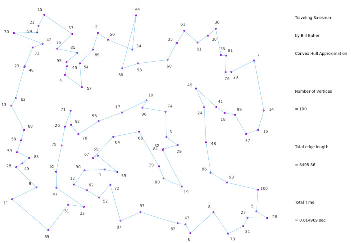
When this 2nd part of the algorithm is finished , you will get the following diagram.
(Click on image for a large version)
The diagram above shows the Convex Hull / Shrink Wrap approximation to a Traveling Salesman path. This approximation has a path length that is only 7.72 % longer than the optimum path - and this could be easily improved by rerouting the edges between vertices 50 and 68. On top of an improved path, the computer code for this algorithm was easier.
Addendum
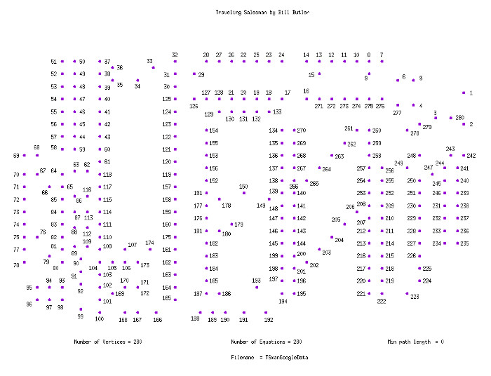
The program was used for a larger data set of vertices that can be accessed at
https://developers.google.com/optimization/routing/tsp
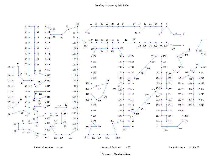
This data set consists of 280 vertices that represent holes to be drilled in a circuit board. "The problem is to find the shortest route for the drill to take on the board in order to drill all of the required holes."
(Click on image for a large version.)
Note: Coordinates for vertices 171,172 are duplicates.
(Click on image for a large version.)
The picture above shows one of the many alternate optimal solutions. The original problem given on "github" lists another of these alternate solutions, but the lower path length given at "github" appears to have not included one edge segment. (For example, the solution at "github" for the path from vertex 191 to vertex 202 plus vertices up to the 140s is different, but the net path length is the same as that given above.)
Once again, the program was able to find the solution in polynomial time without "branch and bound" operations.
Notes on the solution process: Larger problems involve a huge number of possible solutions with multiple near optimal solutions. There is a limit to what computer precision can do. Given the limits of ordinary computational precision, for problems above 1,000 vertices, it may not be possible to exactly determine which solution is optimal; or for that matter, computer arithmetic may not be accurate enough to even find the optimal solution.
Web page generated via Sea Monkey's Composer HTML editor
within a Linux Cinnamon Mint 18 operating system.
(Goodbye Microsoft)
Return to Durango Bill's home page
